Modelling Surface Acoustic Wave Driven Thin Film Flows over Topography

$ \newcommand{\lrp}[1]{\left( #1 \right)} \newcommand{\lrb}[1]{\left[ #1 \right]} \newcommand{\lrc}[1]{\left\{ #1 \right\}} \newcommand{\lrv}[1]{\left\langle #1 \right\rangle} \newcommand{\abs}[1]{\left\lvert #1 \right\rvert} \newcommand{\norm}[1]{\left\lVert #1 \right\rVert} \newcommand{\grad}{\nabla} \newcommand{\bigo}[1]{\operatorname{\mathcal{O}}\!\left(#1\right)} \newcommand{\bigomega}[1]{\Omega\!\left(#1\right)} \newcommand{\vect}[1]{\boldsymbol{#1}} \newcommand{\vecu}{\vect{u}} \newcommand{\deriv}[2]{\frac{d #1}{d #2}} \newcommand{\pderiv}[2]{\frac{\partial #1}{\partial #2}} \newcommand{\pderivtwo}[2]{\frac{\partial^2 #1}{\partial #2^2}} \newcommand{\func}[2]{#1\!\lrp{#2}} \renewcommand{\bar}[1]{\overline{#1}} \newcommand{\cexpz}{e^{2k_i \lrp{x + \alpha_1 z}}} \newcommand{\cexpp}{e^{2k_i \lrp{x + \alpha_1 \phi}}} $

Introduction

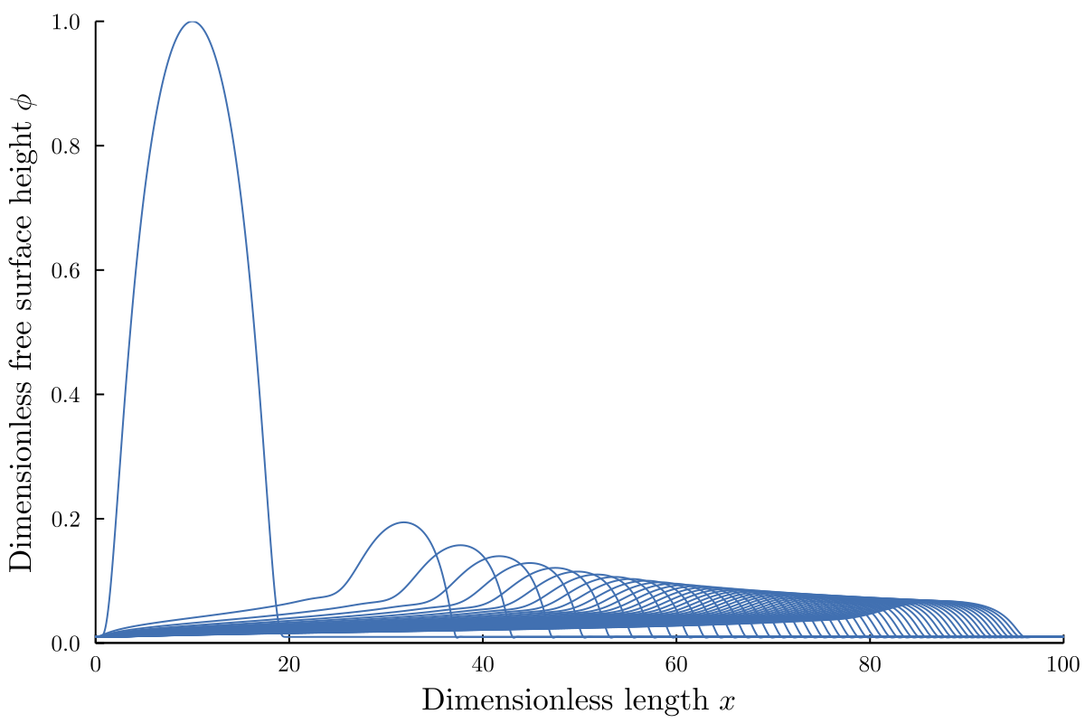
Motivated by the acoustowetting phenomenon and its applications to the dynamic wetting of objects by a coating liquid, we explore the influence of surface acoustic waves and gravity on the motion of a thin film flowing over a surface. We consider surfaces that may be both inclined and include topographical features like trenches, mounds, bumps, etc. Using the lubrication approximation, we reduce the equations of motion for the film to a single nonlinear partial differential equation that describes the evolution of the film height relative to the surface topography in time and space.

Governing Dimensional Equation

We let

• $\func{s}{x, y}$ describe the topography of the surface
• $\func{h}{x, y, t}$ describe the film thickness relative to $\func{s}{x, y}$
• $\func{\phi}{x,y,t} = \func{s}{x, y} + \func{h}{x, y, t}$ be the height of the free surface

We start with the incompressible Navier-Stokes equations $$ \begin{gather} \nabla \cdot \vect{u} = 0 \label{eq:incompress}\\ \rho \lrp{\pderiv{\vecu}{t} + \lrp{\vecu \cdot \grad}\vecu} = -\grad p + \mu \grad^2 \vecu + \rho g \sin \beta \vect{i} - \rho g \cos \beta \vect{k} - \rho J e^{2k_i \lrp{x + \alpha_1 z}} \vect{i} - \rho J \alpha_1 e^{2k_i \lrp{x + \alpha_1 z}} \vect{k} \label{eq:ns-eq} \end{gather} $$ where

• $\vect{u} = \lrp{u,v,w} =$ Fluid velocity, $p =$ Fluid pressure, $\rho =$ Fluid density, $\mu =$ Fluid viscosity
• $k_i =$ Attenuation coefficient, $\alpha_1 =$ Geometric constant, and $J = \lrp{1 + \alpha_1^2}A^2\omega^2 k_i$ is a constant we define to consolidate acoustic forcing terms

Using the lubrication approximation, applying boundary conditions, and depth averaging the resulting vector, we can simplify Eq. \ref{eq:ns-eq} into the following equation for our depth-averaged velocity vector $$ \begin{equation*} \bar{\vect{v}} = -\frac{h^2}{3\mu} \lrp{\rho g \cos\beta \grad \phi - \gamma\grad\kappa - \rho g \sin\beta\vect{i} + \frac{\rho J}{2k_i}\grad \cexpp}. \end{equation*} $$ where $\kappa$ is the curvature of the free surface, $\gamma$ is the surface tension of the liquid, and $\vect{v} = \lrp{u, v}$. Using the depth-averaged conservation of mass $$ \begin{equation*} \pderiv{h}{t} + \nabla \cdot \lrp{h \bar{\vect{v}}} = 0 \end{equation*} $$ and approximating $\kappa = \nabla^2 \phi$ gives us a dimensional equation $$ \begin{equation} \pderiv{h}{t} = \frac{1}{3\mu} \lrb{ \grad \cdot \lrb{\rho g \cos \beta h^3 \grad \phi} - \grad \cdot \lrb{\gamma h^3 \grad\grad^2\phi} - \rho g \sin\beta \pderiv{h^3}{x} + \grad \cdot \lrb{\frac{\rho J}{2k_i}h^3\grad \cexpp}}. \label{eq:thin_film_dim} \end{equation} $$ for the height of the film relative to the surface.

Dimensionless Equation and Simplifications

To transform the dimensional governing equation into a dimensionless one, we use the following scalings $$ \bar{x} = \frac{x}{x_c}, \quad \bar{y} = \frac{y}{x_c}, \quad \bar{z} = \frac{z}{h_c}, \quad \bar{t} = \frac{t}{t_c} $$ for the in-plane coordinates and time where an overline denotes a dimensionless quantity. Additionally, we define $\varepsilon = h_c / x_c$ and define the nondimensional Bond number and Acoustic Weber number as $$ \mathrm{Bo} = \frac{x_c^2 \rho g}{\gamma} \quad \quad \mathrm{We_{ac}} = \frac{\rho \omega^2 A^2 x_c}{\gamma}. $$ Using the scalings and nondimensional parameters, we can manipulate Eq. \ref{eq:thin_film_dim} into $$ \begin{align} \pderiv{h}{t} = \mathrm{Bo} \cos\beta \grad \cdot \lrb{ h^3 \grad \phi } - \grad \cdot \lrb{h^3 \grad\grad^2\phi } - \frac{\mathrm{Bo}}{\varepsilon} \sin\beta \pderiv{h^3}{x} + \frac{\lrp{1 + \alpha_1^2} \mathrm{We_{ac}}}{2\varepsilon} \grad \cdot \lrb{h^3 \grad e^{2k_i \lrp{x + \alpha_1 \varepsilon \phi}}} \label{eq:nondim_final} \end{align} $$ after removing any overlines.

To further simplify the model, we reduce our problem to two spatial dimensions by making the assumption that the free surface of the thin film does not change in the transverse direction (i.e. $h$ and $s$ are both $y$-independent). This reduces Eq. \ref{eq:nondim_final} to $$ \begin{align} \pderiv{h}{t} = \mathrm{Bo}\cos\beta \lrb{h^3 \phi_x}_x - \lrb{h^3 \phi_{xxx}}_{x} - \frac{\mathrm{Bo}}{\varepsilon} \sin\beta \lrb{h^3}_{x} + \frac{k_i \lrp{1 + \alpha_1^2}\mathrm{We_{ac}}}{\varepsilon} \lrb{h^3 e^{2k_i \lrp{x + \alpha_1 \varepsilon \phi}} \lrp{1 + \alpha_1 \varepsilon \phi_x}}_x. \label{eq:two_dim_final} \end{align} $$

Additionally, to enforce that the SAW forcing occurs starting from the film front, we redefine $k_i$ (in dimensionless form) as $$ \begin{align} \func{k_i}{\phi} = x_c \lrp{\lrp{k_i^{\text{oil}} - k_i^{\text{air}}}\lrp{1 - e^{-x_c(\phi-b)/\lambda}} + k_i^{\text{air}}} \label{eq:k_i} \end{align} $$ where $k_i^{\text{oil}}$ denotes the attenuation in the film, $k_i^{\text{air}}$ denotes the attenuation outside the film, and $\lambda$ is a dimensional constant that controls the steepness of the change from $k_i^{\text{air}}$ to $k_i^{\text{oil}}$.

Results

To solve the dimensionless governing PDE, we first discretize it into a system of coupled ODEs. We then use an implicit time stepping scheme called Rodas4 to model to free surface height over time. Additionally, although the governing PDE describes the motion of thin film with both gravity and SAWs as driving forces, we are mainly interested in the case where the SAWs are the primary driving force. Hence, in all our simulations we use $\beta = 0$.

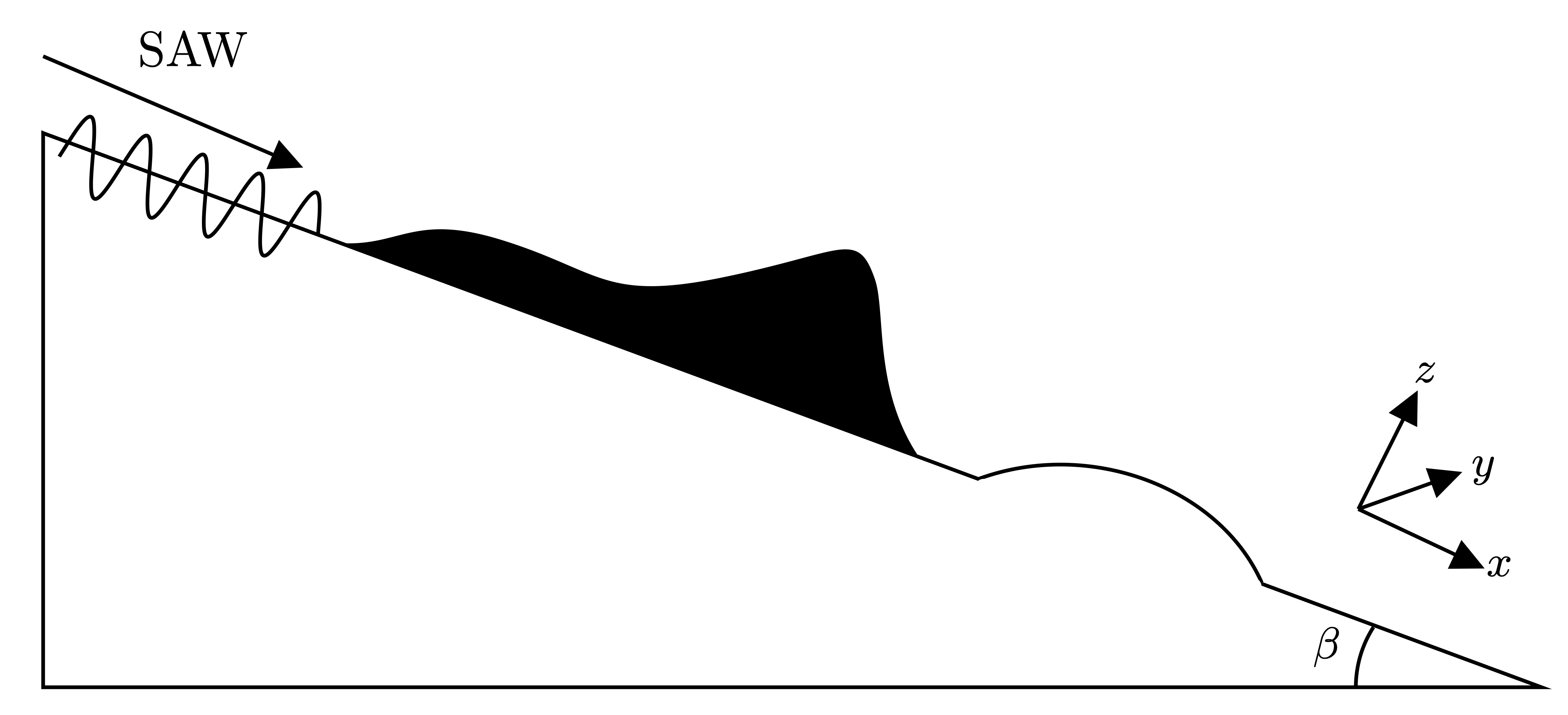
In the case of a flat topography (i.e. $\func{s}{x} = 0$) we find that the initial drop moves from left to right and spreads out as it does so, which matches experimental observations.

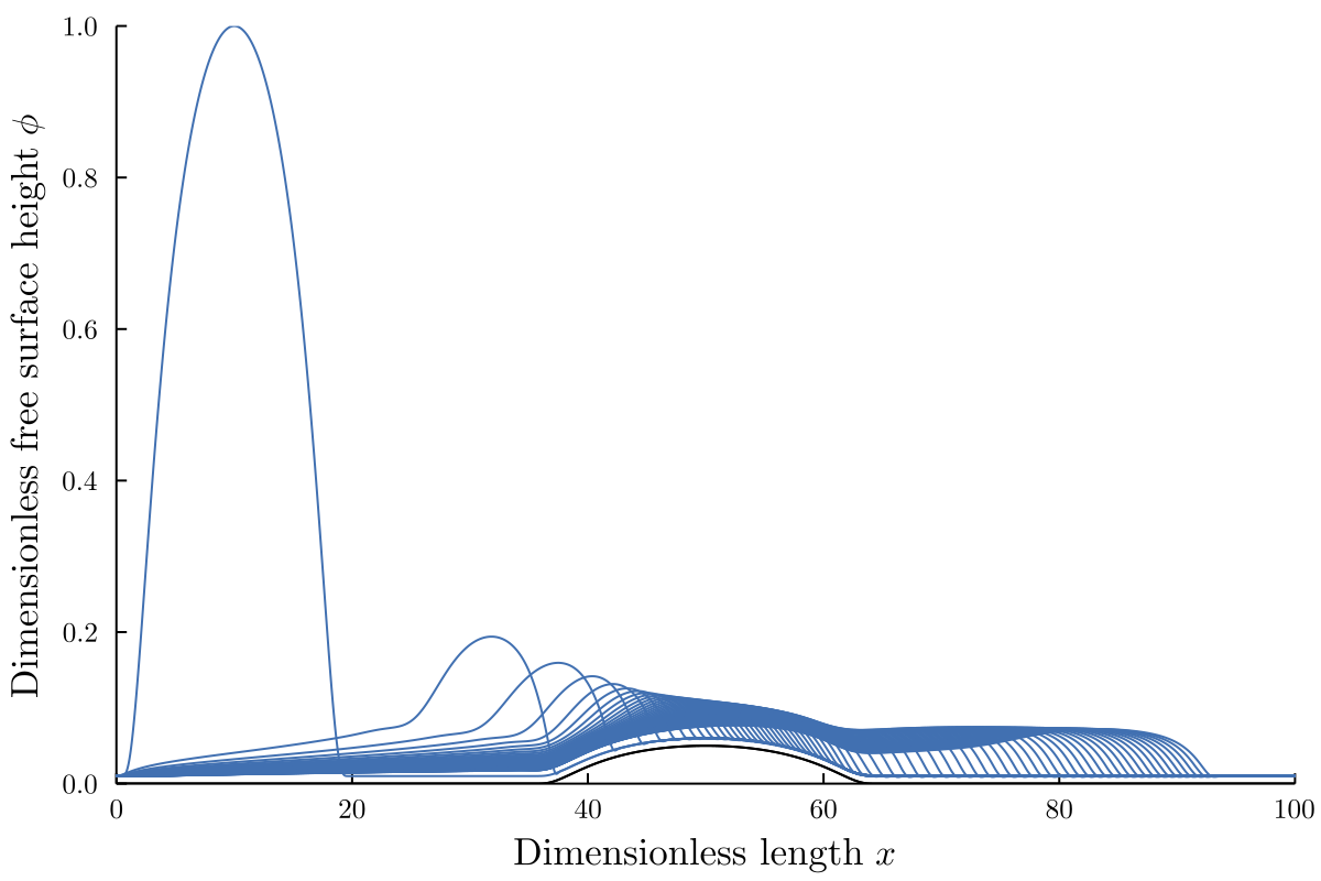
When we introduce a bump topography, we find that if the bump is short enough, the initial drop can clear the bump and spread over the domain as shown below.

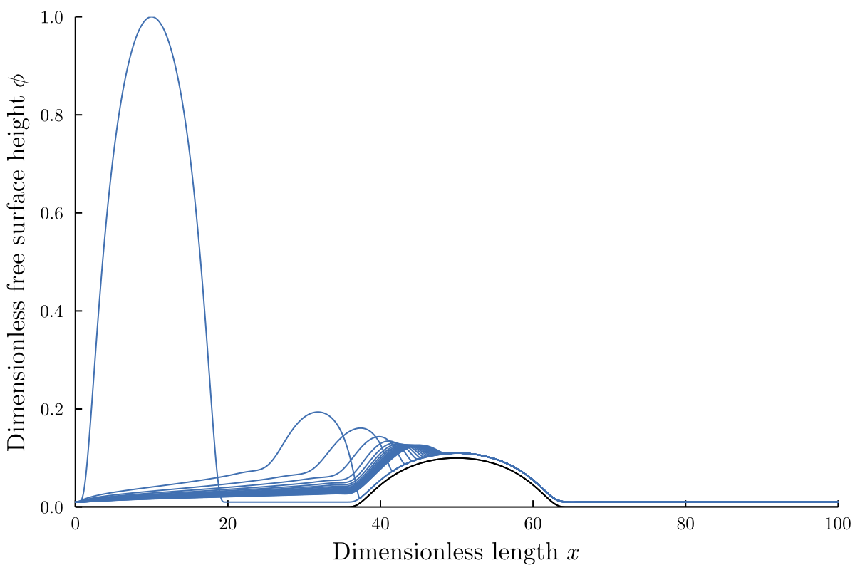
However, when the maximum height of the bump is too large, the fluid gets stuck on the bump as shown below. This behavior makes sense as the SAW travels along $h=0$, so in essence there is no acoustic forcing that can drive the fluid over the bump region.