Over the course of the 2022 Spring semester, we based our project on the spreading thin liquid films with external vibrations, focusing on the works of Dr Kondic, Dr Altshuler, Dr Borcia et al. This model is concerned with determining the effects that vibration parameters such as amplitude and frequency have on the time it takes for a fluid droplet to spread. If you're interested in a full-depth display of what we've worked on, check out our full report.
Supervisor:
Professor Lou Kondic
Lab Assistant:
Joseph D'Addesa
Group Members:
Marina Markaki and
Denisse Mendoza
Acoustics are known to influence fluid motion. Recent experiments were performed in which acoustic driving was used to produce targeted motion of different fluids. This experimental setup involved fluids spreading on substrates. Oil film responds to acoustic driving, while water drops don’t. So in theory, acoustic driving could be used to separate oil and water. The problem of solving coupled partial differential equations (PDEs) is being reduced by considering modeling coupling between fluid motion and acoustics in terms of simplified models.
The original motivation for this project involved simulating a fluid coating another one with a driving force. We approached this simulation by expanding on an easy original problem. We started with a discretized model of a fluid droplet on an angled plane with gravity being the driving force. In an attempt to simulate coating of a fluid, we then added an obstacle to our model. Eventually, we moved to modeling the spreading of a single droplet, by considering a flat plane. Finally, we introduced vertical vibrations on a flat surface and the closing of a hole with said vibrations.
Firstly, we start with the Navier Stokes equation with vibration \[\frac{\partial \bar{u}}{\partial \bar{t}}+(\bar{u}\cdot \bar{\nabla})\bar{U}=-\frac{1}{\rho}\bar{\nabla}\bar{\rho}+\frac{\mu}{\rho}\bar{\nabla}^2\bar{u}-g(1+\epsilon\sin(\bar{\omega t}))\] Then, after imposing boundary and initial conditions we end up with \[\frac{dh}{dt}=-\frac{1}{3\mu}\nabla(\gamma\bar{h}^3\nabla^3\bar{h}-\rho g(1+a(t))\bar{h}^3\nabla \bar{h}+\rho g \bar{h}^3b(t))\hat{i}\] which is the dimensional thin film equation. \(a(t)\) and \(b(t)\) correspond to normal and lateral accelerations respectively, both measured in units of g. In order to nondimensionalize it, we substitute \(x=\frac{\bar{x}}{x_c}\), \(h=\frac{\bar{h}}{h_c}\), \(t=\frac{\bar{t}}{t_c}\) and distributing the negative sign, we end up with \[\frac{h_c}{t_c}\frac{dh}{dt}=\frac{1}{3\mu}\frac{1}{x_c}\nabla(\rho g(1+a(t))h^3h_c^3\nabla h\frac{h_c}{x_c}-\gamma h^3h_c^3\nabla^3h\frac{h_c}{x_c^3}-\rho g h^3h_c^3b(t))\hat{i}\] After combining like terms and dividing both parts with \(\frac{h_c}{t_c}\) and factor out the coefficient on the \(h^3\nabla^3\) term we get \[\frac{dh}{dt}=\frac{\gamma t_ch_c^3}{3\mu x_c^4}\nabla\left(\frac{x_c^2\rho g}{\gamma} (1+a(t))h^3\nabla h-h^3\nabla^3h-\frac{x_c^3\rho g}{h_c\gamma} h^3b(t)\right)\hat{i}\] We choose \(x_c\) so that our last coefficient equals to 1, \(x_c=\left(\frac{h_c\gamma}{\rho g}\right)^{1/3}\). Then we choose \(t_c\) so that our outter coefficient equals 1, \(t_c=\frac{3\mu x_c^4}{\gamma h_c^3}\) which give us \[\frac{dh}{dt}=\nabla\left(\frac{x_c^2\rho g}{\gamma} (1+a(t))h^3\nabla h-h^3\nabla^3h- h^3b(t)\right)\hat{i}\] We let \(D=\frac{x_c^2\rho g}{\gamma}\) , \(a(t)\) equals the amplitude-frequency equation we use in our code \(\epsilon\sin(\omega t)\) and since in our case we are only considering vertical accelerations, we can set \(b(t)\) equal to 0 and remove it from the equation, giving us: \[\frac{dh}{dt}=\nabla\left(D (1+\epsilon\sin(\omega tt_c))h^3\nabla h-h^3\nabla^3h\right)\] Finally we distribute the \(\nabla\) to get the final non-dimensional thin film equation with vibration: \[\frac{dh}{dt}=D (1+\epsilon\sin(\omega tt_c))\nabla[h^3\nabla h]-\nabla[h^3\nabla^3h]\]
Finally, we began exploring the effects of vibrations on the closing of holes. We had to determine how we wanted to mathematically represent the closing of the holes. We decided to track two measures: the time both sides of the fluids take to “touch” and the time they take to “fully close”. Since our initial condition had the hole centered around \(x=50\) , we defined the time to touch as the time it takes for the minimum height to be found at the center. We define the time to close as the time it takes for the maximum and minimum height to have an absolute difference of some tolerance. We chose a tolerance of \(0.05\).
We consider an initial condition of a film that reaches a height of \(1 h_c\) with a film thickness of \(0.1 h_c\). The film expands the \(100 x_c\) length. There is a hole centered at \(x=50x_c\) with a width of \(40 x_c\). We want to compare how long the hole takes to close for constant gravity compared to when vibration is introduced. To simulate constant gravity, we simply made \(\epsilon =0\) and found that the times to touch and times to close were \(628.9\) and \(1646.7 t_c\) respectively. However, interesting things happened when we varied the values of \(\epsilon\). Below is a table showing the different times for changing values of \(\epsilon\).
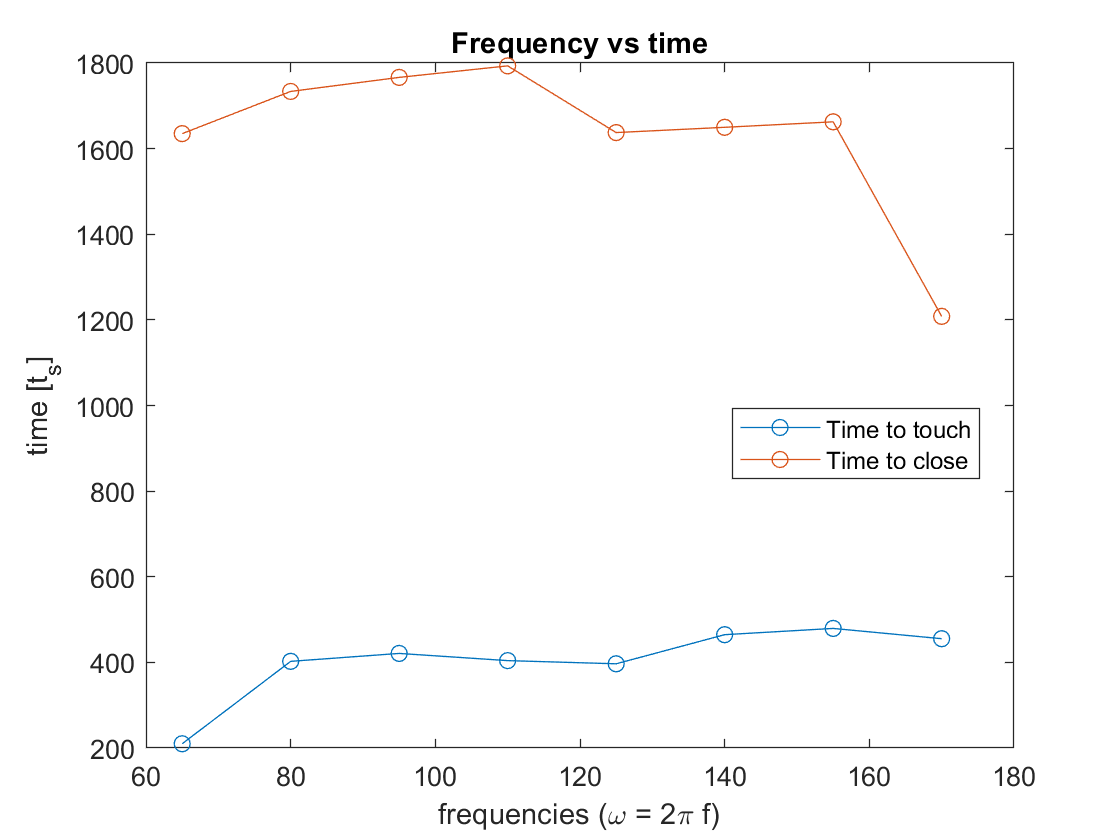
We chose the different values of \(\epsilon\) and \(\omega\), based on our scales. Knowing that angular frequency \(\omega=2 \pi f\) and since it does have a dependency on time, we scaled it down with respect to \(t_c\). That made \(\bar{\omega}=\omega \cdot t_c = 2 \pi f \cdot t_c\) , where \(65\le f \le 170\) came from the experimental results. Since gravity is being multiplied to our amplitude-frequency equation \(1+\epsilon\sin(\omega t)\), amplitude is being scaled down only by \(g\), so \(\epsilon=\frac{a}{g}\), where a, our amplitude, also came from the experimental results. We used \(0\le \epsilon \le 4\), as we had some significant numerical errors for higher values of \(\epsilon\). Below there is a visual representation of how time changes when the values of amplitude and frequency increase.
It’s important to note that for high values of \(epsilon\), we had significant numerical problems, namely, the vibrations were showing very high amplitudes, much higher than the maximum height of our initial condition of the hole. Secondly, we realized that we could have better defined how to represent the touching and closing of a hole. We observed that for certain values of \(\epsilon\) and \(\omega\), the hole appeared to almost close before being “interrupted” by a vibration that increased the amplitudes again. To find a way around this, we could have either increased our tolerance, or redefined our criteria to use a standard deviation as opposed to the difference between the maximum and minimum values.
With that said, our models show a slight relationship between characteristics of a vertically vibrating force and the time a liquid takes to drop and spread. In the \(\epsilon\) vs time figure, it can be seen that a higher amplitude does decrease the time it takes for a hole to close and merge. This doesn’t hold true for \(\epsilon=4\) because at this point, our model started becoming sensitive to the high-amplitude waves. Moreover, the \(\omega\) vs time figure doesn’t show a very clear relationship between the frequency and time to close. We believe this may be due to the way we defined closing and merging, as described earlier.
There is a lot of room for growth here, as we only ever got to analyze the effects of vibration on closing holes that were already unstable. There are models that can be made with stable holes as the initial condition. There can also be an obstacle introduced to the model to see how the vibrations affect spreading in that case. There is also a lot that can be discovered with the introduction of lateral vibrations, which we did not include in our research.