Methodology

Our first objective was to simulate the deposition of a particle on a micro-filtration membrane, an algorithm known as diffusion limited aggregation (DLA) was used. Diffusion limited aggregation is the process of placing a stationary seed in a lattice, then releasing a second seed at a random location. 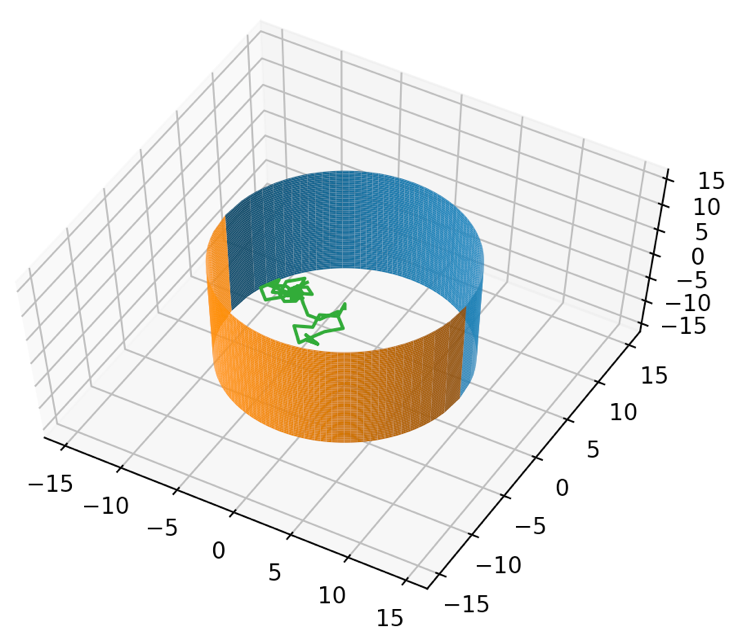At this point the second seed performs a random walk through the lattice until it meets the stationary seed at which point it attaches to it and a new seed is added to again perform a random walk. A lattice is to be initialized and used with a height of 200 grid points and a width of 100 grid points. As the particle moves throughout the lattice it may come in contact with the membrane or other particles that have been attached to the membrane, also known as an aggregate. When the particles touch the membrane or aggregate, it remains in the position depending on an additional parameter, the sticking probability for the membrane (SPM) and the sticking probability for the aggregate (SPA). See Figure 3.1 for an illustration of the membrane.

Fig 3.1

Generating Membrane Profile

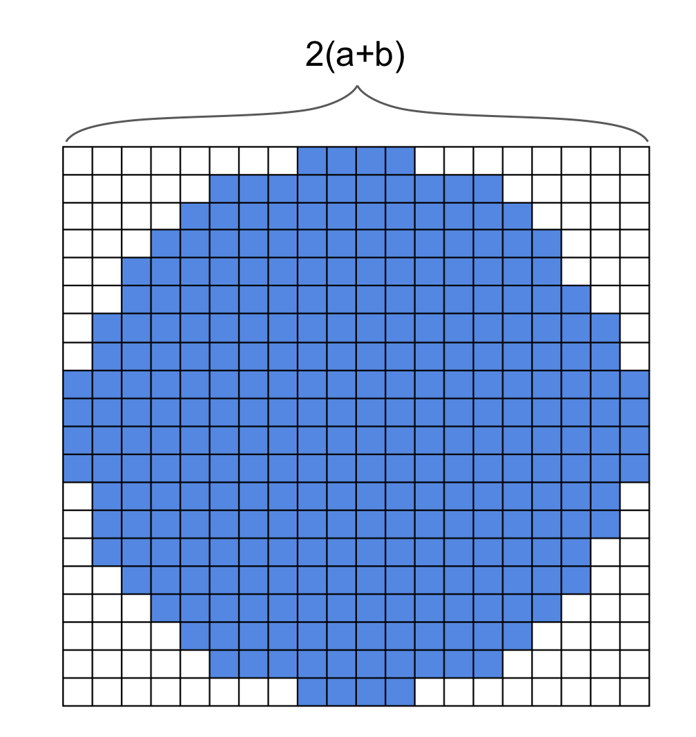
We are particularly interested in morphologies with pore radii that decrease linearly as you traverse the length of the membrane from the pore opening to closing. As such we refer to $A(X,T)$ as the radius of the pore as a function of X (the vertical direction) and T time units where the number of starting particles is our measure for time. According to Darcy`s Model for flow through a porous medium [4] the local membrane resistance is proportional to ${A(X,0)}^{-4}$ where $A(X,0) = aX+b$. This implies that the average membrane resistance (after substituting $u = aX +b$ ) is given by: $$r(t) = \int_{0}^{1} \frac{\,dx}{A(X,0)^4} = \int_{0}^{1} \frac{\,dx}{{(aX+b)}^4} = \frac{1}{a} \int_{b}^{a+b} \frac{\,du}{u^4} \\ = \frac{1}{3a} \frac{1}{u^3} \Big|_{a+b}^b = \frac{1}{3a} \Big ( \frac{{(a+b)}^3 - b^3}{b^3{(a+b)}^3} \Big ) = 1.5$$

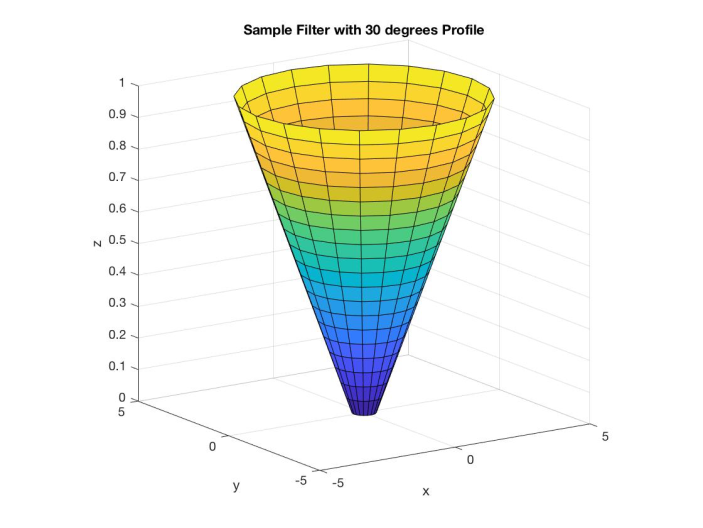
We were able to formulate various pairs of coefficients, a and b, for a range of angles. Using those coefficients we will alter the simulation methodology to generate different membrane profiles. This will be done by implementing the formulation of the membrane as a function of a and b. To begin we must first discretize the geometries of our simulation. The coefficients generated will form a membrane with height of 1, ranging from X = 0 to X = 1, however, for our simulation, we need to generate the membrane for a wider range of X- values. See Figures 3.3 and 3.4

Fig 3.3

Fig 3.4

A STAR Search Algorithm

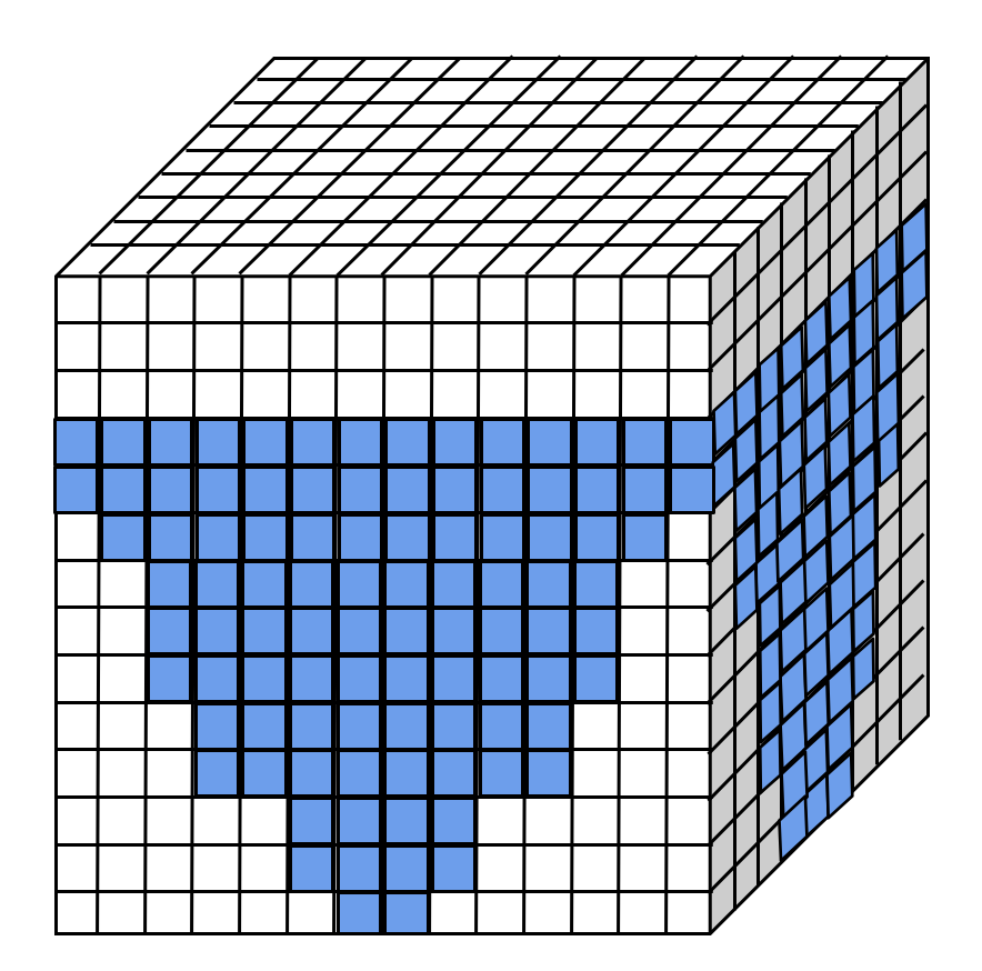
To determine if a pore is clogged, our problem is reduced to a path-finding algorithm; i.e. if we're able to find a path from the top of the lattice to the bottom (through the membrane) then we can conclude that the pore is not clogged. The A* (A STAR) search algorithm is a path finding algorithm that implements heuristic search to efficiently find a path with the least cost [5]. The cost of a node is denoted by $f(n) = g(n) + h(n)$, where $g(n)$ is the cost from the start node to current node n, and $h(n)$ is the heuristic estimate or estimated cost from current node n to the final node. We estimate the h value using the Chebyshev distance with $$h(n) = \text{max(|current.x - goal.x|, |current.y - goal.y|)}$$ X,Y denote their respective X and Y positions on the lattice, and $f(n)$ estimates the lowest total cost of any solution through node n. At each point, the node with the lowest f value is chosen for expansion, and the process repeats itself.
There are a maximum of 8 possible directions in which we can search (in 2D space: up, down, left, right, up-left, up-right, down-left down-right). This yields a branching factor (max possible paths) of 8. The running time of any path-finding algorithm is $O(b^d)$ where b is the branching factor (possible paths) and d is the distance from start to end (pore width). Typically, this results in an exponential run time because each possible path will be fully explored in search of the optimal path. However, the heuristic algorithm like A* looks at the most likely neighboring nodes that would result in a path based on the $f$ value detailed above. In in our case, we are only interested in finding if a pore is blocked or in other words, if a path does not exist. Existence of a path means there is no blocking which is found if a path is found from through the pore.

Fig 3.5

Normal Probability Distribution

To better examine the performance of our filter, we'd like for the particles to be forced through the membrane (using advection flow) via a normal distribution (instead of a typical uniform distribution). Consider the bottom half of a semi-circle with radius $\pi/2$ and centered at the origin. We use this semi-circle to represent a continuous analogous function of the discrete movement of our particle. We'd like to partition the gaussian distribution into 5 distinct regions over an interval $(\pi/2 , \pi/2)$ with each region respectively representing one of the 5 possible directions the particle may travel to. This gaussian distribution will be centered around $\mu = 0$ but with $\sigma$ unknown.
Suppose $X ~ N(\mu,\sigma^2)$ has a normal distribution and lies within the interval $X \in (a,b), -\infty \le a < b \le \infty$. Then $X$ conditional on $a < X < b$ has a truncated normal distribution. Its probability, $f$, for $a \le x \le b$, is given by \begin{equation} f(x;\mu,\sigma,a,b) = \frac{\phi(\frac{x - \mu}{\sigma})}{\sigma\left(\Phi(\frac{b - \mu}{\sigma}) - \Phi(\frac{a - \mu}{\sigma})\right) } \end{equation} Here, $\phi(\xi)=\frac{1}{\sqrt{2 \pi}}\exp\left(-\frac{1}{2}\xi^2\right)$ is the probability density function of the standard normal distribution and $\Phi(\cdot)$ is its cumulative distribution function. $\Phi(x)=\frac{1}{2} \left( 1+\operatorname{erf}(x/\sqrt{2}) \right)$. Using a brute-force method with $a= -\frac{\pi}{2}\, b= \frac{\pi}{2}$ to numerically integrate all possible values $\sigma$ and $\mu=0$ for $f(x; \mu, \sigma, a, b)$; if the absolute value of the integral minus one is less than some tolerance epsilon, then accept that value for $\sigma$. We can therefore conclude that $\sigma \approx 0.9$ and the probabilities are \begin{equation} \int_{-\frac{\pi}{2} + \frac{k\pi}{5}}^{-\frac{\pi}{2} + \frac{(k+1)\pi}{5}} f(x;\mu,\sigma,a,b) \, dx \end{equation} for k=0,1,2,3,4 to move west, southwest, south, southeast, and east respectively.

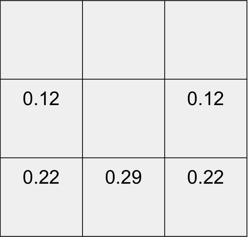
Fig 4.1 Normal Distribution

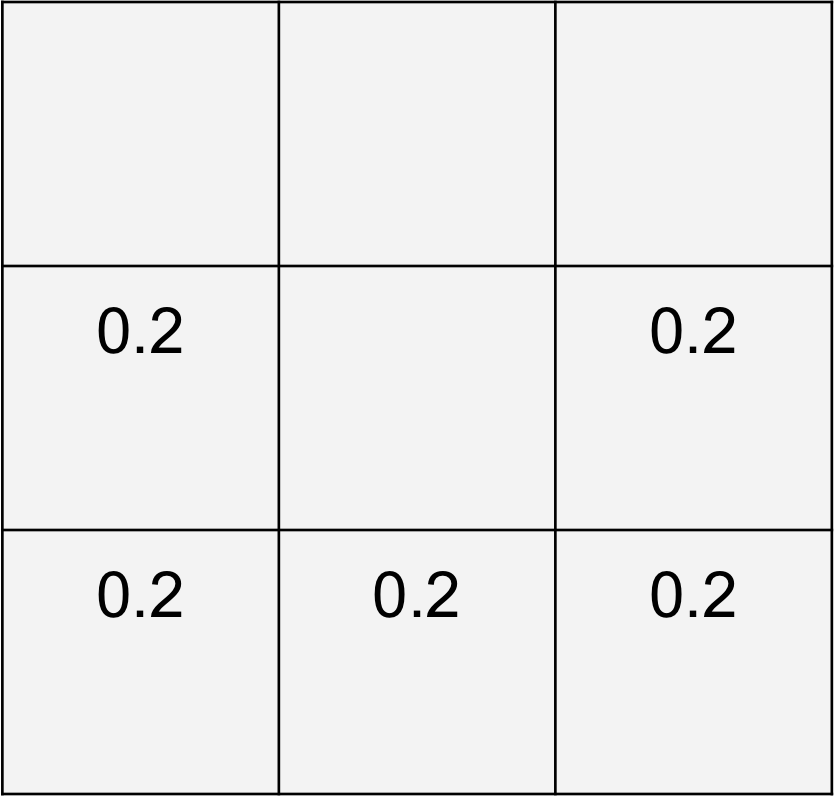
Fig 4.2 Uniform Distribution

Methodology

3D model development progresses in three distinct phases. The first phase involves creating a random walk for a particle without any filter media as if the particle is free to travel in any direction at any point. The second phase introduces the filter media around the particle - at this stage, the filter is very porous and the cylindrical walls of the pores are wide; the particle does not see much boundary action. In the third phase we introduce boundary action by making the media less porous. A less porous media has constricted cylindrical walls of the pores that restrict the random walk of the particles. Attraction forces between the wall and the particle result in particles sticking to the walls and/or to the particles already sticking to the walls, thereby, representing clogging of the filter.

Figure represents end of phase two

Figure represents conical cylinder

Generating Membrane Profile

In this section, we will discuss the creation of the 3D lattice with its characteristic linear profile (which is now modeled as a cone). The lattice will be set to one of 3 integers: 0 denoting an empty space, 1 denoting the membrane, and 2 denoting a particle. Considering strictly the filter (and ignoring creating the empty space above which is trivial) the dimensions of the "cube" will by $[-(a+b),a+b] \times [-(a+b),a+b] \times [0,1]$ where the z-direction (height of the membrane) is given by the interval [0,1]. And the equation for our cone is: $$x^2+y^2 = {(az+b)}^2$$ Note that at z=0, the radius at the bottom of the filter is r=b, and similarly at z=1, the radius at the top of the filter is $r=a+b$. We'll give the z-direction some discrete values i.e. $z_i = hi$ for $i=0,..,N$ and $h=1/N$ where N denotes the resolution of our grid. We can iterate over all $z_i$ and fix the equation of the membrane to be: \begin{equation} {x}^2 + {y}^2 \geq {(az_i + b)}^2 \end{equation} After fixing $z_i$, we similarly discretize the x- and y-direction using the relationship in (8), setting the lattice =1 if this relationship is satisfied, otherwise setting the lattice =0. Using this logic, we can create the membrane and extend the z-direction to include the empty spaces to initialize our particle.